
Every measurement in your physics experiment will have some noise. How can we measure it, and what can we do to deal with it?
Welcome back to the series of posts on experimental error! In the first post, we began to explore some of the ways even a fairly simple experiment is prone to unavoidable experimental error. In this post, we will outline techniques that you can use to mitigate the effects of these unavoidable errors and be able to state the result of your measurement with more certainty. Whether you are taking your first high school physics course, studying physics in college, or submitting a paper to Science, you need to think about the uncertainties inherent in the experiments you perform.
In our experiment, we are trying to measure g, the acceleration due to gravity, by dropping a ball and measuring both the height from which we drop it and the time it takes to hit the ground. Thinking about how we measure the fall time, we came to realize that even such a simple act as timing a falling ball with a stopwatch is prone to significant error! If the average human reaction time is around 0.2 s, how are we supposed to measure an event that only takes 0.6 s with a high degree of reliability?
We started to think about our various sources of error and to make assumptions regarding each, but in the end, our result is only as valid as the assumptions we make to justify it. When designing and carrying out an experiment, we should sit down and think through all of our sources of error – What can go wrong? How important is each source of error? Which will dominate our uncertainty and which can be neglected? – but we need to measure these errors to be completely sure of our result.
Let’s look at various methods we can use to measure and quantify our errors. As with many aspects of designing an experiment, the effort you make to understand and mitigate your measurement error is a matter of judgment; you might not need to go to the lengths described below for your average high school or introductory college lab course, but I want to give some indication of a few commonly used analysis methods.
Get the noise out
Again considering the act of timing the ball’s drop with a stopwatch, we come to realize that there are two types of contributions to our error.
The first contribution is noise. Noise, or random error, is random and varies from run to run. We’ll always be late triggering the stopwatch after the ball hits the ground, but we might be a bit slow on one run and a bit faster on another. As a result, the time we measure and the value of g we calculate will be a bit higher on one run and bit lower on another.
Fortunately, noise is relative easy to deal with. We can reduce the effect that noise has on our result by averaging many runs. If you drop the ball many times and compile a list of the times that you measure, then you will notice that they fluctuate around some central value from drop to drop. The more drops that we average, the better we will know this central value. If we take the list of N drops, then the mean, given by
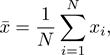
gives our best estimate for the true drop time, and the standard deviation, given by
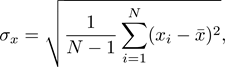
gives a measure of the noisiness of our measurement.
How much should I average?
Great! So the more times I do the experiment and the more data points I average, the better my results will be. Does that mean that if I take enough data points, I can eliminate noise completely? Well, in the words of my advisor, one should be a bit careful.
The more data points we average, the more accurate our estimation for the true drop time becomes, but the precision of our measurement is still limited by noise. This is a subtle distinction, so let’s illustrate the point.
In the following figure, I’ve simulated dropping the ball 3, 30, and 300 times using a theoretical true value of 0.650 s, and plotted histograms of the results.
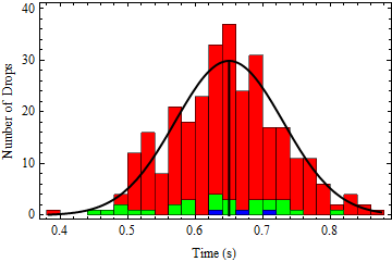
With 3 drops (blue), you just see three data points, which seem to be randomly distributed in the neighborhood of 0.650 s (the vertical black line). With 30 drops (green), you start to see that there’s a spread of points centered roughly around 0.650 s or so. With 300 drops (red), however, you can see clearly that the data points form a distribution centered at 0.650 s. The means of the three data sets are 0.673 s (3 points), 0.631 s (30 points), and 0.648 s (300 points).
As we can see in the data, the more data points we collect, the more confident we can be that the mean of the data set is close to the true value; that is, our result becomes more accurate. No matter how many data points we collect, however, the data will always have some finite spread due to the fact that our measurement apparatus, our trigger finger in this case, is just noisy and imperfect; that is, our precision is still limited by noise.
So, if acquiring more data won’t help forever, when should we stop? Most sources of noise result in the points you measure having some specific distribution around the true value. As we can see in the figure, data that initially looks random begins to form into a pattern as we acquire more and more points.
Once we have enough data to fit it to a specific shape – I chose to model our noise as a normal distribution (the black curve outlining the data) because a surprisingly wide variety1 of things in everyday life exhibit this type of noise – we can make much more powerful statements about our result. For instance, if we found that our data fit a normal distribution well, we could say something like “the most likely actual value is x, and we are 95% certain that the actual value is between y and z.”
More interestingly, the shape of our noise can sometimes give us meaningful information about its physical source. Several noise sources, such as variation in the human response time, follow an approximately normal distribution, but several others do not. If, as we collect our data, we start to see that its shape does not match a normal distribution, then that’s a good clue that something other than our slow trigger fingers is responsible for our noise.
Up next: Bias!
We now understand how we can take care of the noise inherent in our measurement, but noise is only half the story. We can acquire data for days, fit our results beautifully to the normal distribution, and make iron-clad statistical statements about the most likely value and our 95% confidence interval, but how do we know that the result of our measurement and averaging accurately reflects what we are trying to measure? How do we know that we aren’t making some mistake in carrying out the experiment that makes every time we measure either higher or lower than it should be?
Imagine you want to know the average height of a male, high school basketball player. You could measure the height of every player in America and the data would likely form a beautiful curve, but if you forgot to ask every player to take off his sneakers first your data would still be skewed. The number you wind up with, despite your enormous sample size and careful attention to statistics, would not give you the average player’s natural height.
This brings us to the second contribution to our measurement error: bias, noise’s more pernicious cousin. Bias, or systematic error, skews all of your data points in one direction or the other. Bias is generally more difficult to detect and to correct for than noise, and we will discuss several methods that can be used to mitigate its effects in our next blog post.
[1] You can find the normal, or Gaussian, distribution popping up to describe such diverse phenomena as the quantum mechanical vibration of a diatomic molecule, standardized test scores, monthly rainfall, and even the Plinko board from “The Price is Right.”
Comments