In this post, I start off by explaining the Marginal Rate of Substitution (Sections II-IV). Then, I cover the concept of Marginal Utility (Sections V-VII). In both cases, I start with a story explanation, then give a formal definition, and finally provide some other useful information about the concept. After that, I connect the two concepts (Marginal Utility and Marginal Rate of Substitution) and show how they relate mathematically, first without calculus (Section VIII) and then with calculus (Section IX). Finally, I demonstrate that the Marginal Rate of Substitution has an advantage over Marginal Utility in terms of describing preferences and behavior (Section X), because it is less sensitive to the exact utility function you choose to use!
Story Explanation of the Marginal Rate of Substitution
Let’s imagine that I have some jelly beans and some M&Ms. I like both types of candy and I like having the choice between fruity and chocolatey, so I’m pretty happy right now. Now imagine someone comes along and wants one of my jelly beans. Maybe this person only wants half a jelly bean. The point is that the person wants a very very small amount of jelly beans.
If I give the person half a jelly bean, I’m a little less happy than I was before. But! The person could give me some amount of M&Ms that would make me exactly as happy as I was before I gave up that tiny bit of jelly beans. The amount of M&Ms that would make me exactly as happy might be one-third of an M&M, it might be two M&Ms, or maybe it would be half an M&M. The point is, a very small amount of M&Ms would make me equally as happy as I was before, and this amount of M&Ms is not necessarily equal to the amount of jelly beans I gave up.
The Marginal Rate of Substitution captures the rate at which I would be willing to exchange a tiny bit of jelly beans for M&Ms.
Formal Definition of the Marginal Rate of Substitution
The Marginal Rate of Substitution (MRS) is the rate at which a consumer would be willing to give up a very small amount of good 2 (which we call x2) for some of good 1 (which we call x1) in order to be exactly as happy after the trade as before the trade.
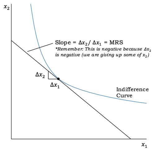
Let ∆x1 and ∆x2 be very small changes (e.g. “marginal” changes) in x1 and x2. Then, the MRS equals ∆x2 ÷ ∆x1. Note that the MRS is negative, because we are giving up some of x2 (so ∆x2 is negative) to get some of ∆x1 (so ∆x1 is positive). A negative divided by a positive is a negative, so it follows that the MRS is negative.
Relationship Between the MRS and Indifference Curves
At any given point along an indifference curve, the MRS is the slope of the indifference curve at that point. Note that most indifference curves are actually curves, so their slopes are changing as you move along them. That means that the MRS is also changing!
To find the slope of a curve at a specific point, you use calculus. Take the first derivative of the equation for the indifference curve, then plug in the values of x1 and x2 for the point you are interested in. That will give you the MRS at that point.
What do you think happens to the MRS along the indifference curve? When I have a lot of x2, I’m willing to give up quite a bit of x2 to get a little bit of x1. However, this changes as I move along my indifference curve. When I get to a point where I’m just as happy as before but now I have tons of x1 and almost no x2, I no longer want to give up much x2 to get a little x1. This phenomenon is known as the diminishing rate of marginal substitution.
The Marginal Rate of Substitution (MRS) is the slope of the indifference curve
Story Explanation of the Marginal Utility
Let’s imagine again that I have some jelly beans and some M&Ms. If someone takes a tiny (“marginal”) amount of jelly beans away from me, I’m slightly less happy. Similarly, if someone gives me a tiny bit more jelly beans, I’m a little happier. My marginal utility of jelly beans is the change in happiness I experience from a tiny (e.g. “marginal”) change in the amount of jelly beans I have.
Similarly, my happiness (which economists call “utility”) would change if someone changed the amount of M&Ms I had. When the change in M&Ms is tiny (“marginal”) then the resulting change in my utility is known as my marginal utility of M&Ms.
Note that in both cases, marginal utility is defined with respect to a specific type of candy that I have. We considered the marginal utility of jelly beans and the marginal utility of M&Ms. We can combine these ideas to figure out what would happen if I experienced simultaneous changes in the amount of jelly beans and M&Ms in my possession, but marginal utility is always defined with respect to a specific good.
Formal Definition of Marginal Utility
The marginal utility with respect to good 1 is the change in utility a consumer experiences when the amount of x1 the consumer has changes by a tiny bit while the amount of x2 the consumer has remains constant. We can represent this marginal utility as:
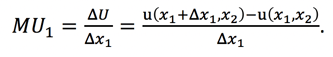
Here, MU1 is the rate of change in utility (∆U) resulting from a small change in good 1 (x1).
Similarly, the marginal utility with respect to good 2 is the rate at which utility changes when the consumer’s amount of x2 is changed by a marginal amount while his/her amount of x1 remains fixed at a constant amount. The equation for MU2 is:
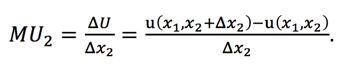 .
.
Marginal utility will always be positive when we are dealing with goods (as opposed to bads or neutrals). This is because getting more will make us happier, so when the denominator (∆x1) is positive, the numerator (∆U) is also positive. Similarly, when we lose some of good 1, ∆x1 is negative and we are less happy, so ∆U is also negative. A negative divided by a negative is positive, so the marginal utility of a good will always be a positive value.
Marginal Utility v. Actual Change in Utility
Note that in both cases, we can do a little algebra to find the total change in utility resulting from a marginal change in one good while the amount of the other good is held constant.
Let’s use good 1 as our example. Above, we saw this:
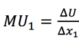
If we multiply both sides by ∆x1, we then have:
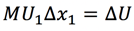
Therefore, the change in utility resulting from a tiny change in good 1 and no change in good 2 is just the product of that tiny change in good 1 and the marginal utility with respect to good 1.
Connection Between Marginal Utility & Marginal Rate of Substitution
The Marginal Rate of Substitution looks at the balance in changes of good 1 and good 2 required for the consumer to be indifferent between his/her consumption bundles before and after trade. But what does indifference mean? It means that utility for both bundles is exactly equal. Therefore, 
There is some (negative) change in utility resulting from giving up a little bit of good 2, and as we saw in the previous section, this change equals 
Similarly, there is some (positive) change in utility from getting a little more of good 1, which equals:

Since we want to be indifferent before and after the trade, it must be that the sum of these changes equals zero. Our equation would thus look like this:
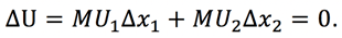
With a little algebra, we can find the MRS from this equation of marginal utilities!
First, when we subtract MU1∆x1 from both sides, we are left with the following, 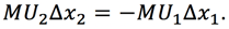
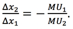
Next, divide both sides by ∆x1 and MU2. The result is
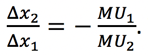
The left hand side is just the MRS, and the right hand side is the negative ratio of marginal utilities. In the MRS section, we learned why the left hand side would automatically be negative. The right hand side needs the negative sign because marginal utility is positive for goods, so the ratio of marginal utilities is always positive.
MRS and Marginal Utility Relationship: Calculus Edition
When using calculus, the marginal utility of good 1 is defined by the partial derivative of the utility function with respect to ∆x1. That is: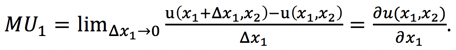
We want to consider a tiny change in our consumption bundle, and we represent this change as(dx1, dx2). We want the change to be such that our utility does not change (e.g. du = 0). Therefore, we want to solve: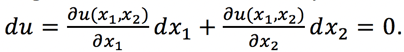
Rearranging terms as before, we find this:
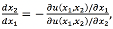
The equation above is just the calculus version of this:
Instead of using derivatives, we could use implicit functions. Any given indifference curve can be represented as
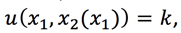
where k is a constant and the level of utility held constant along the indifference curve. We use the notation x2(x1) simply to illustrate that x2 is a function of x1.
If we differentiate both sides of the equation with respect to x1, we get: 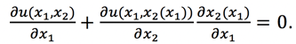
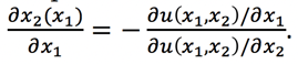
We can again rearrange terms and the result is the same as what we found before:
Monotonic Transformations Affect MU but Not MRS
The downside of marginal utility is that its magnitude depends on the utility function we’re using. This is not ideal, because utility functions are usually ordinal, which means we don’t care exactly what numbers the utility function spits out, we just care that the utility function gives us higher numbers for bundles the consumer likes better.
The great thing about the MRS is that even though it is function of the marginal utilities with respect to goods 1 and 2, it doesn’t change if apply a positive monotonic transformation to our utility function. (Positive monotonic transformations are any functions that preserve the original order when applied, like adding a constant to the original utility function, raising the original utility function to an odd power, taking the natural log, etc.) To see why this is so, let’s pretend u(x1,x2) was our original utility function and is our monotonically transformed utility function (so ƒ(u) is a monotonic function). Then, using our calculus definition of the MRS, we have the following before the transformation:
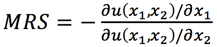
After the transformation, we have:

So the MRS is completely unchanged by any monotonic transformation!
Acknowledgments: much of this post was inspired by chapters 3 and 4 of Hal Varian’s textbook Intermediate Microeconomics: A Modern Approach.
Comments