Welcome to Finance 101! Today we'll cover the time value of money, annuities, and perpetuities.
Introducing the Time Value of Money
Let’s say you have the following choice:
- Receive $100 today
- Receive $100 five years from now
Which option would you pick?
Most people would prefer to receive $100 today (option A). This intuition highlights the time value of money, a fundamental principle that underpins nearly all financial decisions and calculations. The principle states that a dollar today is worth more than a dollar tomorrow.
To deconstruct why this is the case, we must understand that money received today can be invested and grown to a larger amount in the future. In a world where positive investment opportunities exist, the value of a dollar today will be greater than the value of a dollar in the future.
Understanding How Rate of Return Impacts the Time Value of Money
Now, let’s say you have a different set of options:
- Receive $100 today
- Receive $150 five years from now
Which option would you pick?
In this case, the answer would depend on which investment opportunities exist. For example, if you could invest your money at a 5% return each year over a five-year period, would you pick option A or B? What about a 10% return?
To solve this problem, we should think of money as having a “time unit” indicating when it is received or paid. We must compare money in the same time units. To standardize time units, we use the following tools:
- Discounting: converts money back in time
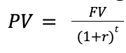
(i.e., “Present Value Formula”)
- Compounding: converts money forward in time
![]()
(i.e., rearrangement of the Present Value Formula)
In the equations above:
- PV = present value of money
- FV = future value of money
- r = annual rate of return on investment opportunity (also known as “discount rate,” “interest rate,” or “opportunity cost of capital”)
- t = time in years
We can use these equations to solve the previous problem. In our example, PV = $100, FV = $150, and t = 5 years. The return on investment (r) remains an unknown variable.
Let’s say r = 5%. If that's the case, we can examine our two options:
- Option A: FV = $100 * (1 + 0.05)5 = $127.63
- Option B: FV = $150
Here, it makes sense to pick option B. The future value of option B ($150) is greater than the future value of option A ($127.63).
Let’s say r = 10%. If that's the case, we can examine our two options:
- Option A: FV=$100 * (1 + 0.10)5 = $161.05
- Option B: FV = $150
In this case, it makes sense to pick option A. The future value of option B ($150) is less than the future value of option A ($161.05).
To generalize, we can solve for the breakeven point to understand when it makes sense to pick option A versus B. To do this, we set PV = FV and solve for r:
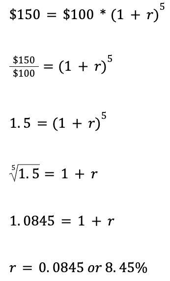
Thus, if the return from the potential investment opportunity is greater than 8.45%, we should pick option A (i.e., take the $100 today and invest it). However, if the return is less than 8.45%, we should pick option B.
(Note: in the example above, it does not matter if we use the discounting or compounding equation, as they are rearrangements of the same formula. The important thing is to make sure that we are comparing money in the same time units – either both in the present, or both in the future.)
In the real world, determining the appropriate rate of return for an individual or company requires significant analysis by finance professionals. The appropriate “r” varies based on factors such as risk profile and available investment opportunities. Key approaches to determine the correct discount rate for a company include computing the firm’s weighted average cost of capital (“WACC”) and cost of equity using the capital asset pricing model (“CAPM”). This post will not go into the details of WACC or CAPM, but it is important to note that robust methodologies exist to determine “r.”
Variations to the Present Value Formula
Variation #1 – Perpetuities
Imagine this: instead of receiving cash at a single moment in time, what if you were to receive a series of cash flows indefinitely? This is known as a perpetuity.
Under a perpetuity, the cash flows (“C”) are regular and constant, and t = ∞. The present value equation would simplify to the following: PV = c/r .
In the real world, an example of a perpetuity is a perpetual bond, which pays interest to bondholders indefinitely.
Let’s say there is a bond that pays $10 coupons each year (with no maturity date) and has a discount rate of r=5%. What would be a fair price to pay for the bond today?
- Would you be overpaying or underpaying if the bond cost $180 today?
- What if the bond cost $220 today?
We can solve this problem by using the perpetuity equation to compute the bond’s present value:
PV = $10/(0.05) = $200
In this case, a fair price for the bond would be $200. We would be underpaying if the bond only cost $180 today (a steal!) and overpaying if the bond cost $220.
Variation #2 – Annuities
What if you were to receive a series of cash flows over a finite time horizon? This is known as an annuity.
Under an annuity, the cash flows (“C”) remain regular and constant, but t is no longer . The present value equation for an annuity is as follows:
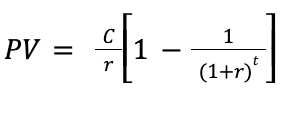
In the real world, common annuities include mortgage payments, lease payments, and some types of retirement income.
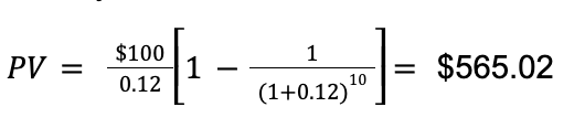
Let’s look at an example: what would be the present value of a lease obligation assuming you pay $100 each year for 10 years at an interest rate of r = 12%? We can solve for this using the annuity formula:
Conclusion
The time value of money is one of the most crucial building blocks of finance. Perpetuities and annuities are simple variations of the present value formula. Understanding these concepts is critical, as nearly all advanced finance analyses build on these fundamental ideas.

Comments