Understanding a confusion matrix

One of the major tasks in machine learning and statistical testing is classification. In classification problems, we use a training set of labeled data to train our model to classify an unlabeled observation into one category or another. At the simplest level, this method uses observable data to make a related yes-or-no classification (like: will it rain today or not rain today). Classification problems can also have more than two classifications (like: will it be cloudy, sunny, rainy, snowy, etc.), but the principles for analyzing the results are largely the same. Many popular techniques exist for classification problems, such as logistic regression, trees (including boosted trees and random forests), and neural networks. To see how well a given method works, we can use a confusion matrix to understand the results of the model.

The Confusion Matrix

The picture below shows a typical layout of a two-class classification with the actual class on the top and our model’s predicted class on the side. In most cases, the matrix shows the number of cases in each of the four cells. Ideally all of our data would fall into the diagonal green cells, and none into the off-diagonal red cells, but models are never that accurate. Instead it is important to understand what each of the different types of errors mean to your problem using medical diagnosis as an example.

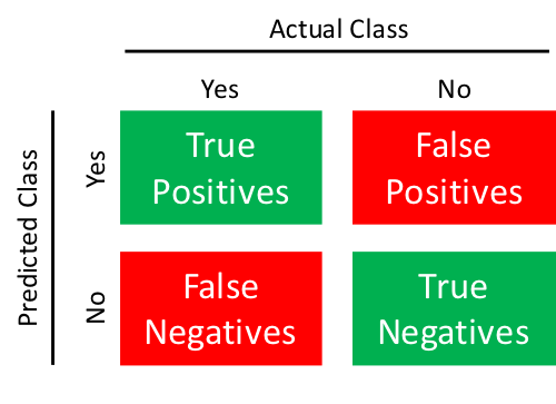
False Positives: Your model classified this individual as having the disease when in reality she was healthy. This is called a type I error and in statistical hypothesis testing is equivalent to rejecting a true null hypothesis.

False Negatives: Your model classified this individual as being healthy when in reality he had the disease. This is called type II error and is equivalent to failing to reject a false null hypothesis.

The Terminology

For me, this is the most confusing part of the confusion matrix. For every possible ratio of numbers, there is at least one fairly ambiguous name describing it. Here are some of the highlights where FP stands for false positive (and so on for TP, FN, TN).

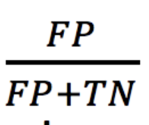
False Positive Rate

This measures how often somebody from the negative population is classigied as positive. In our example, this answer the question: what fraction of healthy people does our model say have the disease? We represent FP with the following equation:

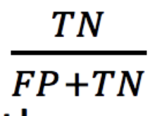
True Negative Rate (or Specificity)

This is one minus the false positive rate and answers the question: what fraction of healthy people does our model say are healthy? We can represent it as follows:

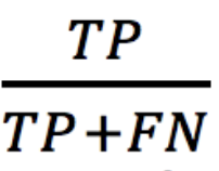
True Positive Rate (also Sensitivity, Recall, or Probability of Detection)

This measures the effectiveness of identifying people who actually have the trait your model tries to detect. Of the people who have the disease, what fraction does you model identify as having the disease. We can represent it as follows:

There are many other statistics used to summarize the matrix, and you can pick the one that makes the most sense for your problem.

Some Examples

Let’s look at two examples to see how the tradeoffs between the two types of misclassification errors.

Hair Length: Imagine you ask somebody the length of their hair then try to determine whether they are female or not female. If their hair is neck-length or longer, you guess female and if its shorter, you guess not female. This is a pretty straightforward model that would work reasonably well. For a 1,000,000 people, your confusion matrix might look like this:

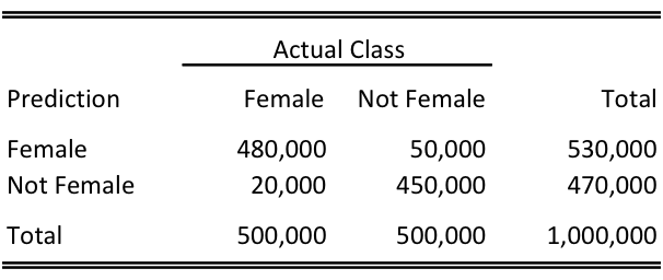
You miss women who wear their hair short (including very young children), and men who have their hair long. Importantly, the population is very balanced between females and not, and there is not an inherent asymmetry in the cost of classifying someone who is not female as female or a vice-versa. Therefore, we can set a middle-of-the-road cutoff like neck length to minimize the total number of incorrect predictions.

Medical Diagnosis: Let’s turn our attention back to medicine and imagine we are testing for a rare disease. You have a very good test (the false positive and false negative rates are both 0.1%), but for a very rare disease (also 0.1%). Your confusion matrix might look like this:

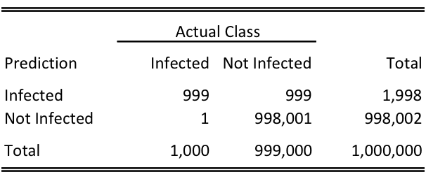
In these types of tests we have two key differences from the hair example: an unbalanced population and unbalanced costs of error. First, there are many more uninfected people than infected, and second, a false negative could lead to an untreated disease and very high costs, while a false positive could be fairly easily remedied, say, by running another test. In this case, we may want to accept a high false positive rate in exchange for minimizing the false negative rate to address these cost asymmetries.

We also have the curious result due to the unbalanced population that, if tested at random, a positive test result gives you a 50% probability of having the disease. But, that is a topic for another blog post about conditional probability.