Where do Taylor series come from and why do we learn about them?

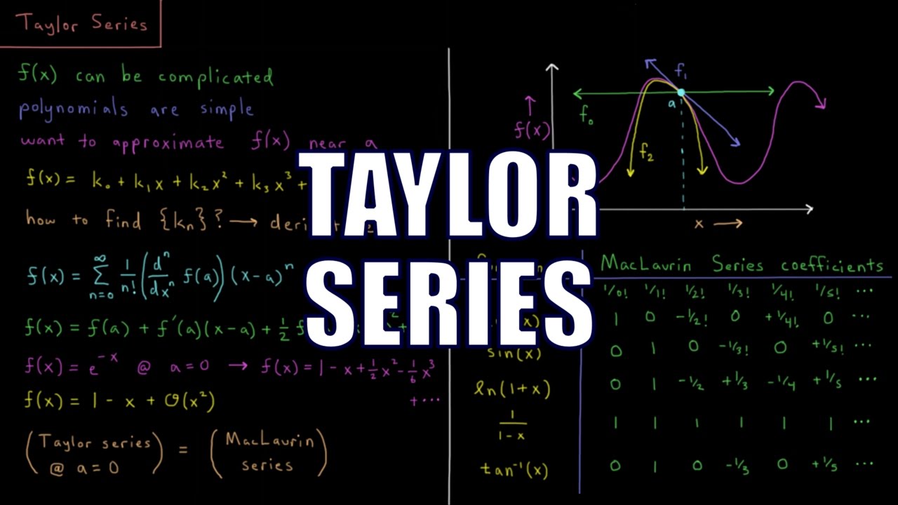
Taylor series can often seem a bit mysterious the first time that we learn about them. The formula for the Taylor series of a function f(x) around a point x=a is given by

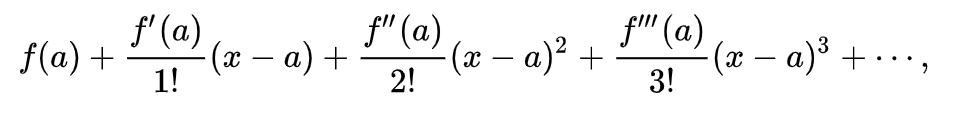
where ƒ(n)(a) denotes the nth derivative of the function f(x) at x=a. To compute a Taylor series, we find the nth derivatives and substitute them into the formula.

But what is a Taylor series really? Taylor series are an incredibly important tool for numerical approximation. In this post, we’ll break down the motivation for Taylor series and shed some light on where they come from.

A starting point: linear approximations

One of the simplest types of functions that we can have are linear functions, those of the form y=mx+b. Linear functions are easy to graph and to evaluate.

Suppose that we have a complicated function like f(x)=cos(x) that is hard to evaluate precisely without a calculator. Suppose now that we wanted to estimate the value of cos(x) near x=0. One way that we could do this is with a linear approximation. That is, we will construct a linear function g(x)=mx+b that is close to f(x)=cos(x) at x=0. To do this, we should think about what values of b and m give us the best approximation of f(x)=cos(x).

Well, since we are looking for an approximation near x=0, a good starting point is to have g(x)=f(x) at x=0. That is, since cos(0)=1, we want g(0)=m(0)+b = 1, and so b=1. To figure out what value of m works best, we want g(x) to be tangent to f(x) at x=0, so the slope m should be equal to f’(0) = -sin(0) = 0. This gives us g(x) = 1 as our linear approximation.

We can see f(x)=cos(x) as the red curve below and g(x) = 1 as the blue curve below.

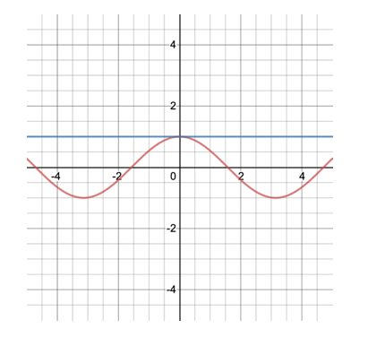
From the graph above, we see that for x close to zero, g(x)=1 is a reasonable approximation of cos(x). That is, cos(x) for very small values of x is close to 1. But this approximation is not very good for larger values of x.

How can we make our approximation better?

An improvement: quadratic approximations

The linear approximation g(x) = 1 for f(x) = cos(x) didn’t take into account any of the curviness of the graph of cos(x). If we wanted to capture the curviness in our approximation, but still wanted to keep our approximation simple, the correct thing to do is to approximate f(x) = cos(x) not by a linear function, but by a polynomial.

Let’s start by trying to approximate f(x) = cos(x) near x=0 with a quadratic polynomial

What’s the best that we can do here? Well, like in the linear case, we still want g(0) = f(0). Since g(0) = a and f(0) = cos(0) = 1, this gives us that a=1.

We also want the first derivatives g’(0) = f’(0) to capture the slope of the tangent line of the graph near x=0. This gives us that b = -sin(0) = 0, and so b=0.

Let’s also try to ensure that the second derivatives of g(x) and f(x) match at x=0. The second derivative determines the rate of change of the derivative, and so matching the second derivatives will roughly give us that the graphs of f(x)=cos(x) and of our approximation g(x) curve at the same rate around x=0.

Since the second derivative of g(x) at x=0 is g’’(0)=2c and the second derivative of f(x) = cos(x) at x=0 is f’’(0) = -cos(0) = -1, this gives us that 2c=-1, and so c = -1/2.

As a result, our quadratic approximation is:

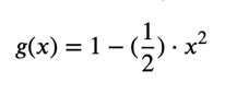
If we plot f(x) = cos(x) in red and our approximation g(x) in blue, we get the following graph:

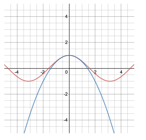
We see that this our quadratic approximation is indeed a better approximation of our original function near x=0

Higher order approximations

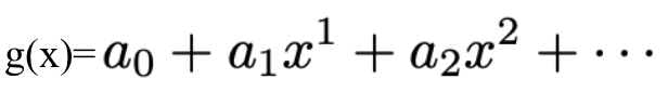
But there's no reason to stop here! We could continue approximating our function f(x) = cos(x) with polynomials of higher and higher degrees. Let g(x) equal the following:

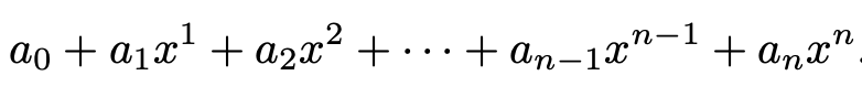
With this equation, let's match the values of the first n derivatives of g(x) at x =0 with the corresponding derivatives of f(x) at x=0.

What is the mth derivative of g(x) at x=0? Well, with some thought we can see that if m is at most n, then the following equation is true:

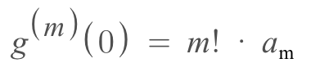
This tells us that we should have:

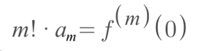
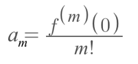
Written another way, we have:

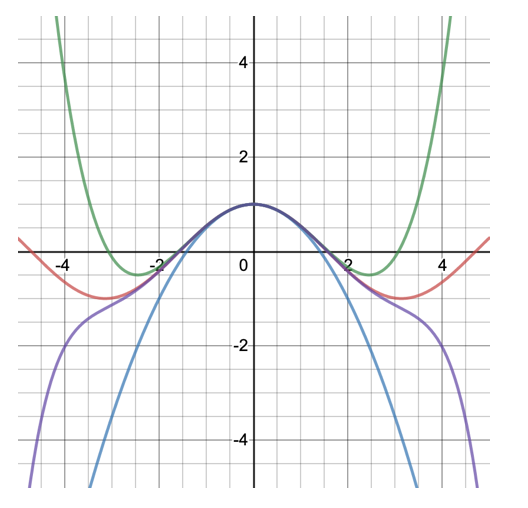
In the below graph, we see f(x) = cos(x) graphed in red, and some better and better polynomial approximations found in this way:

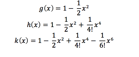
graphed in blue, green, and purple respectively.

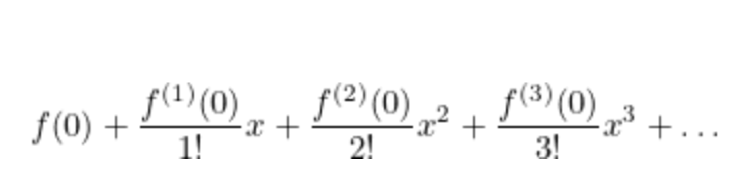
If we continue this process indefinitely, then what we get is a Taylor approximation:

For f(x) where the mth derivatives of f(x) and g(x) to match at x = 0, we need to bring in:

If we rearrange the terms, we see that:

This gives us that formula for the Taylor series around x=0 (sometimes also known as the Maclauren series) of a general function f(x).

General Taylor series formula

To finish off this discussion, we note that sometimes we want to approximate a function f(x) near a point x=a where a is not necessarily zero. Then, we need to shift this whole discussion to be centered around x=a rather than x=0.

To do this, we match the derivatives of our function f(x) and our Taylor series not at x=0, but at x=a. Doing so, we find that the correct approximation is our original Taylor series expression from the beginning of this post.

So there were have it! We started at linear approximations, moved on to polynomial approximations, and ended on Taylor series, which are in a way infinitely good polynomial approximations.

Whenever we want to approximate a complicated function numerically, we can take the first few terms of the Taylor series expansion of the function to get a nice polynomial approximation. The more terms we take, the better approximation we get. This relationship to polynomial approximations is just one of the many properties of Taylor series that make them such a useful and powerful mathematical tool!