One of the most important equations in econometrics – and in economics in general – is the equation for omitted-variable bias. This simple equation is a powerful tool for reasoning about the ways in which correlations we see in the data may differ from the causal relationships we care about. In this post, we'll begin by learning exactly what the omitted-variable bias equation is and where it comes from. Then we'll learn why the equation is so important and how to use it when interpreting data.
The Omitted-Variable Bias Equation
The omitted-variable bias equation relates the coefficients from three different linear regressions. It applies no matter what the dependent and independent variables are, but to make things concrete, let's focus on the relationship between income and education.
First, let's consider estimating a simple regression of individual income on years of school completed:
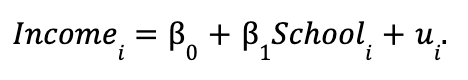
This regression relates the income of person i to the number of years they were in school. We'll call this regression the "short regression" because there's only one independent variable, Schooli.
Now suppose we also observe data on whether person i was born in a high-income ZIP Code. Now we could estimate a linear regression model that controls for each person's background:
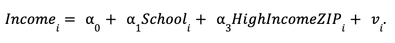
Here, HighIncomeZipi is a binary variable that equals 1 if person i was born in a high-income ZIP Code. Because we've added another independent variable, we'll call this the "long regression.”
Finally, let's consider estimating a regression that relates each person's background to the number of years they go to school:
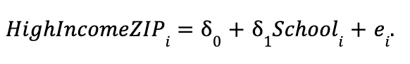
This regression is called the "auxiliary regression".
We're now ready to define the omitted-variable bias equation! The equation is:
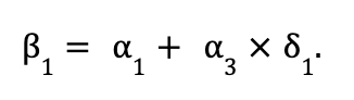
In words, the equation says that the coefficient on Schooli from the short regression is equal to the coefficient from the long regression plus a bias term. The size and sign of the bias depends on the relationship between Schooli and the outcome, Incomei, as well as the relationship between Schooli and the omitted variable, HighIncomeZipi.
This equation is simple enough to memorize, but it's worth taking a moment to think about why the expression makes sense. From our long regression, we know that being born in a high-income ZIP Code is associated with an increase in income of 3. And from the auxiliary regression, we know that each additional year of school is associated with an increased probability of being from a high-income ZIP Code of 1 percentage points. So if we don't control for HighIncomeZIPi, then an additional year of school is associated with an increase in income that is directly related to school, 1 and an increase in income that comes from the fact that one more year of school is associated with an increase in HighIncomeZIPi of 1. In other words, omitting HighIncomeZIPi leads to some of the relationship between a person's background and their income to be attributed to their years of school.
As a final step to understanding the equation, we can derive it from our three regression equations. We start by substituting the auxiliary regression into the long regression and rearranging:

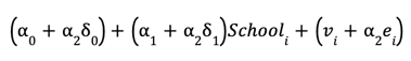
Notice that substituting in the auxiliary regression eliminates the variable HighIncomeZIPi, leaving us with Schooli as the only independent variable, just like in the short regression. By rearranging the expression, we have three distinct sets of terms: a constant, the variable Schooli multiplied by a slope coefficient, and a residual term. This mirrors the structure of the short regression equation, and the different terms are in fact exactly identical to what you would get if you simply estimated the short regression.
Using the Omitted-Variable Bias Equation: Correlation and Causation
The omitted-variable bias equation describes a general statistical relationship between any short and long regression. But the equation is most powerful when used to think about a short regression that describes a correlation in the data and a long regression that describes a causal relationship. Let's stick with our example of education and income, specifying a short, long, and auxiliary regression, but this time let's consider a different omitted variable:
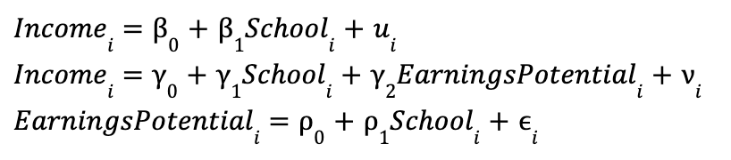
Now our omitted variable is EarningsPotentiali, which measures how much money person i would earn if they only stayed in school long enough to graduate from high school. It's reasonable to think that if we could control for an individual's earnings potential, then the relationship we would observe between income and school would be causal. That is, the regression coefficient y1 represents the average causal effect of an additional year of school on earnings!
So, what does the omitted-variable bias equation say in this case? Writing out the expression, we have:

That is, the correlation between education and income that we see in the data represents the causal impact of additional years of school on income and a bias term. What's more, we can use this expression to reason about the direction of the bias. To do so, we need only ask ourselves what we think the sign of the coefficients y2 and p1 are. So, what do you think? Is earnings potential positively or negatively correlated with income? Is it positively or negatively correlated with years of schooling?
If you suspect that people with higher earnings potential make more money and attend school longer, then both y2 and p1 are positive, which means that the bias, y2 x p1, is positive. That is, the relationship we see in the data between school and income is biased upwards relative to the true causal effect, since people who stay in school longer also have higher earnings potential. On the other hand, if you think that people with higher earnings potential make more money but complete less school (maybe because they drop out to start a successful tech company), then p1 is negative and the bias, y2 x p1, is also negative. So the relationship we see in the data between school and income is biased downward relative to the true causal effect, since people who stay in school longer have lower earnings potential.
One powerful thing about using the omitted-variable bias equation in this way is that it allows you to think about omitted variables that you don't actually observe in your data and that you never would be able to observe in real data. EarningsPotentiali is a perfect example of this -- there is no dataset of hypothetical earnings for people if they only finished high school. But we can still reason about how this unobservable variable would be correlated with the variables that we do observe, and this helps us understand how our regression estimates differ from the causal effects we're interested in.
Practice
For economists, applying the omitted-variable bias equation to think about how a regression estimate might be biased is second nature, but it comes from years of practice. Consider the following patterns in the data and try using the omitted-variable bias equation to reason about whether these patterns represent causal relationships or not. If not, do you think the true causal effect is larger or smaller than the observed correlations?
- People in the hospital on average have worse health than people who aren't in the hospital.
- Drinking green smoothies is associated with better heart health.
- Students who go to a professor's office hours get better grades on average.
- States with higher minimum wages have lower average unemployment.
- Neighborhood housing costs tend to go up when new luxury apartments are built.

Comments